#1 Chromatin remodeling induced by IFN-α
Mireia Ramos-Rodríguez
Details
Original publication:
Colli, M.L., Ramos-Rodríguez, M., Nakayasu, E.S. et al. An integrated multi-omics approach identifies the landscape of interferon-α-mediated responses of human pancreatic beta cells. Nat Commun 11, 2584 (2020). https://doi.org/10.1038/s41467-020-16327-0
Contents: Analyses and figures contained in this document correspond to the following figures/sections of the original publication:
- Results: “Interferon-\(\alpha\) induces early changes in chromatin accessibility”.
- Figure 1: “Exposure of EndoC-\(\beta\)H1 cells to interferon-\(\alpha\) promotes changes in chromatin accessibility, which are correlated with gene transcription and translation”. Panel b.
- Supplementary Figure 3: “Gained open chromatin regions are mainly localized distally to gene transcription starting sites (TSSs), evolutionary conserved and enriched in transcription factors (TFs) binding motifs”. Panels a, b and c.
- Additional quality control measures requested during the Review process.
Analysis of ATAC-seq data
Quality control
Run Rscript for generating the necessary quality control measures.
Rscript code/IFNa_QC_ATAC.R# Get RSC and NSC indexes
# source("QC_phantom_peak.R") # Runs code to generate files
load("../data/IFNa/ATAC/QC/QC_scores.rda")
sc <- txt[,c("sampleID", "NSC", "RSC")]
# Load alignment stats
load("../data/IFNa/ATAC/QC/summary.rda")
stats <- sum.df[!grepl("_2$", sum.df$samples),c("samples", "al.raw", "perc.align", "perc.filtOut")]
colnames(stats) <- c("sampleID", "Lib Size", "% Align", "% Mito")
nms <- unique(stats$sampleID)
lvl <- rev(nms[c(grep("ctrl-2h", nms),
grep("ctrl-24h", nms),
grep("ifn-2h", nms),
grep("ifn-24h", nms))])
stats <- dplyr::left_join(stats, sc)
stats$sampleID <- factor(stats$sampleID,
levels=lvl)
lib_size <-
ggplot(stats,
aes("Lib Size", sampleID)) +
geom_tile(aes(fill=`Lib Size`), color="black", size=.3) +
geom_text(aes(label=round(`Lib Size`/1e6, 2))) +
scale_fill_gradient(low="white", high="darkorchid4",
limits=c(0, max(stats$`Lib Size`)),
breaks=c(0, max(stats$`Lib Size`)),
labels=c("0", "Max"),
name=expression("Library size (x"*10^6*")"),
guide = guide_colorbar(direction="horizontal",
title.position = "bottom",
title.vjust = 1,
title.hjust = 0.5,
label.position = "top",
label.vjust=0,
label.hjust = c(0,1),
frame.colour="black",
frame.linewidth = 0.7,
ticks=FALSE)) +
theme(legend.position = "bottom",
axis.title = element_blank(),
axis.ticks.x = element_blank(),
axis.line = element_blank())
align <-
ggplot(stats,
aes("% Align", sampleID)) +
geom_tile(aes(fill=`% Align`), color="black", size=.3) +
geom_text(aes(label=round(`% Align`, 1))) +
scale_fill_gradient(low="white", high="darkorange3",
limits=c(0, max(stats$`% Align`)),
breaks=c(0, max(stats$`% Align`)),
labels=c("0", "Max"),
name="% alignment",
guide = guide_colorbar(direction="horizontal",
title.position = "bottom",
title.vjust = 1,
title.hjust = 0.5,
label.position = "top",
label.vjust=0,
label.hjust = c(0,1),
frame.colour="black",
frame.linewidth = 0.7,
ticks=FALSE)) +
theme(legend.position = "bottom",
axis.title = element_blank(),
axis.ticks = element_blank(),
axis.line = element_blank(),
axis.text.y = element_blank())
mito <-
ggplot(stats,
aes("% Mito", sampleID)) +
geom_tile(aes(fill=`% Mito`), color="black", size=.3) +
geom_text(aes(label=round(`% Mito`, 1))) +
scale_fill_gradient(low="dodgerblue3", high="white",
limits=c(0, max(stats$`% Mito`)),
breaks=c(0, max(stats$`% Mito`)),
labels=c("0", "Max"),
name="% mitochondrial",
guide = guide_colorbar(direction="horizontal",
title.position = "bottom",
title.vjust = 1,
title.hjust = 0.5,
label.position = "top",
label.vjust=0,
label.hjust = c(0,1),
frame.colour="black",
frame.linewidth = 0.7,
ticks=FALSE)) +
theme(legend.position = "bottom",
axis.title = element_blank(),
axis.ticks = element_blank(),
axis.line = element_blank(),
axis.text.y = element_blank())
nsc <-
ggplot(stats,
aes("NSC", sampleID)) +
geom_tile(aes(fill=NSC), color="black", size=.3) +
geom_text(aes(label=round(NSC, 1))) +
scale_fill_gradient(low="white", high="brown3",
limits=c(1, max(stats$NSC)),
breaks=c(1, max(stats$NSC)),
labels=c("1", "Max"),
name="NSC",
guide = guide_colorbar(direction="horizontal",
title.position = "bottom",
title.vjust = 1,
title.hjust = 0.5,
label.position = "top",
label.vjust=0,
label.hjust = c(0,1),
frame.colour="black",
frame.linewidth = 0.7,
ticks=FALSE)) +
theme(legend.position = "bottom",
axis.title = element_blank(),
axis.ticks = element_blank(),
axis.line = element_blank(),
axis.text.y = element_blank())
rsc <-
ggplot(stats,
aes("RSC", sampleID)) +
geom_tile(aes(fill=RSC), color="black", size=.3) +
geom_text(aes(label=round(RSC, 1))) +
scale_fill_gradient(low="white", high="aquamarine4",
limits=c(1, max(stats$RSC)),
breaks=c(1, max(stats$RSC)),
labels=c("0", "Max"),
name="RSC",
guide = guide_colorbar(direction="horizontal",
title.position = "bottom",
title.vjust = 1,
title.hjust = 0.5,
label.position = "top",
label.vjust=0,
label.hjust = c(0,1),
frame.colour="black",
frame.linewidth = 0.7,
ticks=FALSE)) +
theme(legend.position = "bottom",
axis.title = element_blank(),
axis.ticks = element_blank(),
axis.line = element_blank(),
axis.text.y = element_blank())
plot_grid(lib_size,
align,
mito,
nsc,
rsc,
nrow=1,
rel_widths=c(0.3, rep(0.175, 4)),
align="h")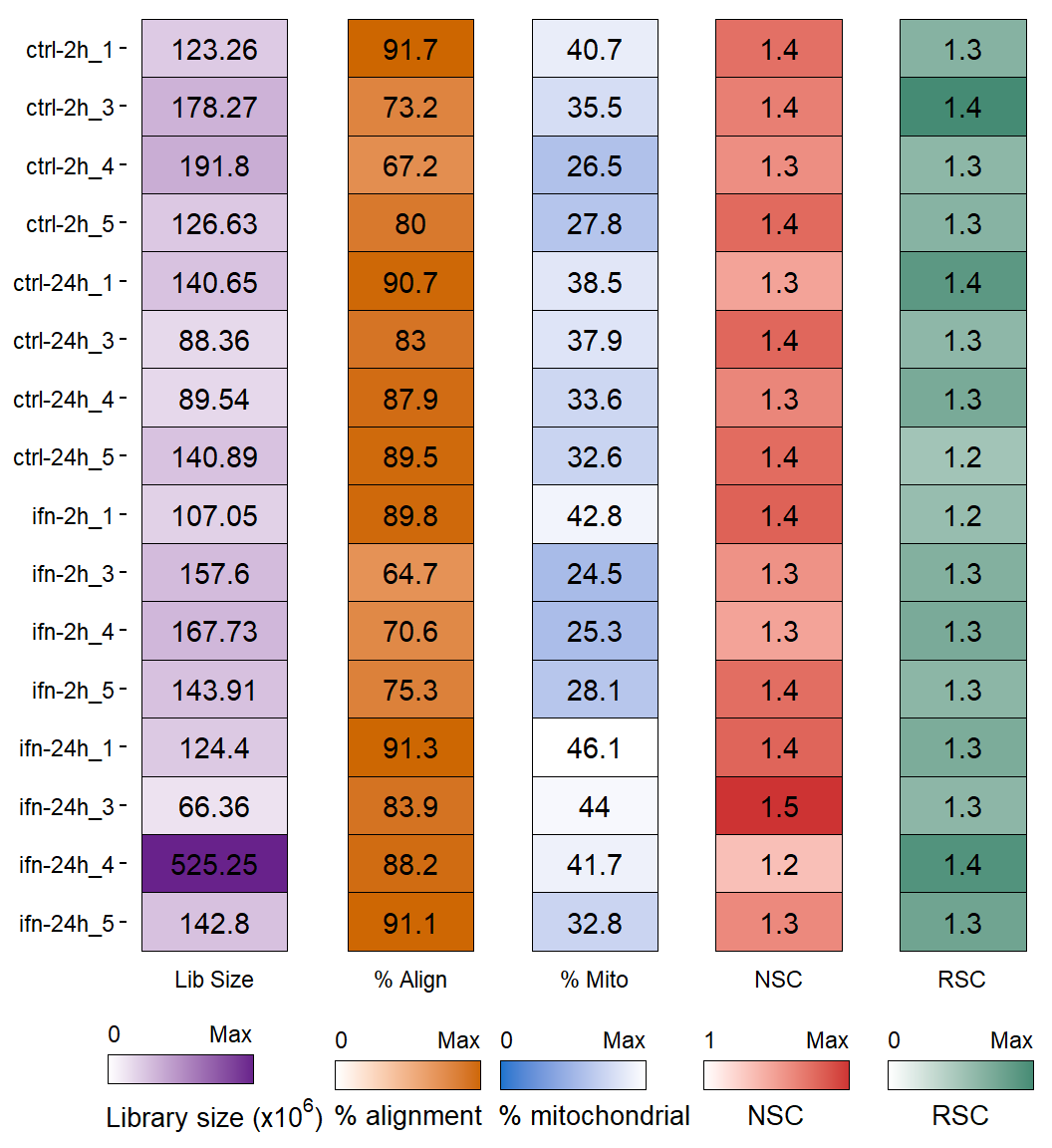
Figure 1: Sumary of per-replicate sequencing metrics, showing total library sizes, percentage of aligned reads, percentage of mitochondrial aligned reads, normalized strand cross-correlation coefficient (NSC) and relative strand cross-correlation coefficient (RSC).
load("../data/IFNa/ATAC/QC/ATAC_tss_enrichment.rda")
tss <- enr

tss$dataset <- factor(tss$dataset, levels=c("TSS annotation", "Random control"))
tss$group <- factor(tss$condition,
                        levels=c("ctrl-2h", "ctrl-24h", "ifn-2h", "ifn-24h"),
                        labels=c("'Control 2h'", "'Control 24h'",
                                 "'IFN-'*alpha*' 2h'", "'IFN-'*alpha*' 24h'"))
tss <- tss %>%
  group_by(dataset, group, Position) %>%
  summarise(mean=mean(mean))

tss.plot <-
  ggplot(tss,
       aes(Position, mean)) +
  geom_line(aes(group=dataset, color=dataset), lwd=0.7) +
  scale_color_manual(values=c("seagreen4", "goldenrod3"), name="Dataset") +
  facet_wrap(~group, scales="free_y", labeller= label_parsed) +
  theme(legend.position="top") +
  ylab("Mean ATAC-seq read counts") + xlab("Position relative to TSS (bp)")

tss.plot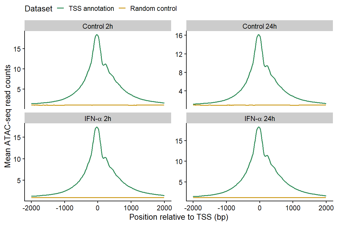
Figure 2: Enrichment of ATAC-seq reads around protein-coding TSS compared to a randomized set of regions.
load("../data/IFNa/ATAC/QC/ATAC_noise.rda")

stats$condition <- factor(stats$condition,
                              levels=c("ctrl-2h", "ifn-2h", "ctrl-24h", "ifn-24h", "Random"),
                              labels=c("'Ctrl 2h'", "'IFN-'*alpha*' 2h'",
                                       "'Ctrl 24h'", "'IFN-'*alpha*' 24h'", "Random"))

noise <-
  ggplot(stats[stats$Annotation!="Unassigned",],
       aes(condition, mean)) +
  geom_bar(aes(fill=Annotation), stat="identity",
           position="stack",
           color="black", lwd=0.7) +
  geom_errorbar(aes(ymin=cumsum, ymax=cumsum+sd,
                    group=Annotation),
                width=.3, lwd=0.5) +
  scale_fill_manual(values=c("violetred", "dark orange")) +
  scale_y_continuous(name="Percentage of reads in peaks (%)") +
  scale_x_discrete(labels=function(x) parse(text=x)) +
  theme(axis.text.x=element_text(angle=30, hjust=1),
        legend.position="top",
        axis.title.x=element_blank())

noise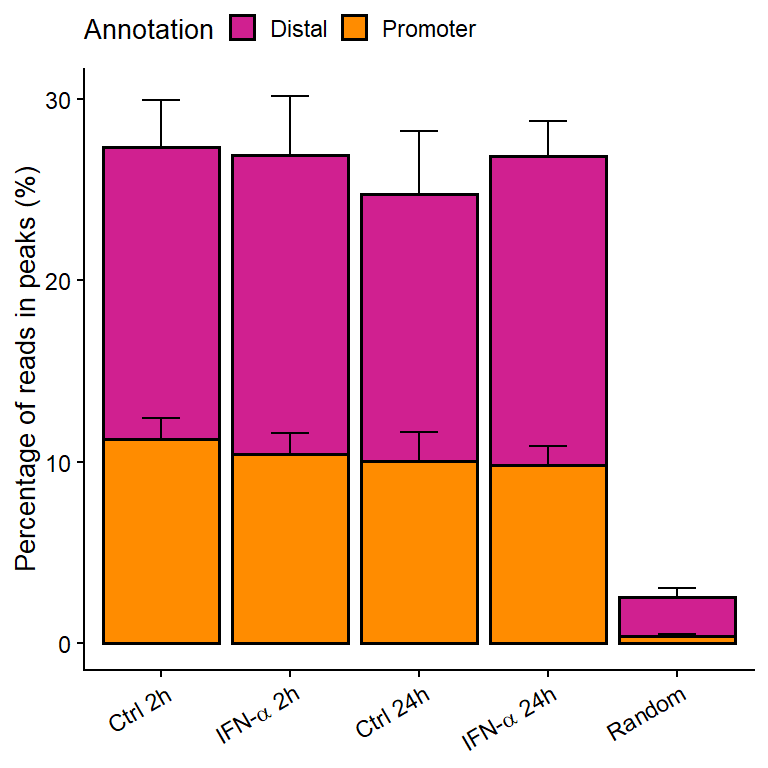
Figure 3: Signal-to-noise ratios of ATAC-seq reads located at called peaks vs reads outside peaks.
 get_upper_tri <- function(cormat){
    cormat[lower.tri(cormat)]<- NA
    return(cormat)
 }

  get_lower_tri <- function(cormat){
    cormat[upper.tri(cormat)]<- NA
    return(cormat)
  }
load("../data/IFNa/ATAC/QC/ATAC_10kb_correlation_rsubread.rda")
mat <- cor(counts$counts, method="pearson")
mat[lower.tri(mat, diag=FALSE)] <- NA
df <- reshape2::melt(mat)
df <- df[!is.na(df$value),]
df$condition <- gsub("_[[:digit:]]", "", df$Var1)
df <- df[gsub("_[[:digit:]]", "", df$Var2)==df$condition,]
df$condition <- factor(df$condition,
levels=c("ctrl-2h", "ctrl-24h", "ifn-2h", "ifn-24h"),
labels=c("'Ctrl 2h'", "'Ctrl 24h'",
"'IFN-'*alpha*' 2h'", "'IFN-'*alpha*' 24h'"))
ggplot(df,
aes(Var1, Var2)) +
geom_tile(aes(fill=value), color="black", size=.7) +
geom_text(aes(label=round(value, 2)), color="white") +
scale_fill_gradient2(low="white", high="royalblue4",
mid="steelblue2", midpoint=0.5,
limits=c(0,1),
breaks=scales::pretty_breaks(n=3),
name="Pearson's correlation",
guide=guide_colorbar(title.vjust = 1,
label.hjust=0.5,
label.vjust=1,
frame.colour="black",
frame.linewidth=.7)) +
facet_wrap(~condition, scales="free", labeller=label_parsed) +
theme(axis.title=element_blank(),
axis.text.x=element_text(angle=30, hjust=1),
legend.position="bottom",
legend.justification="center",
axis.line=element_blank(),
strip.background = element_rect(fill="white",
color="black", size=.7,
linetype=1))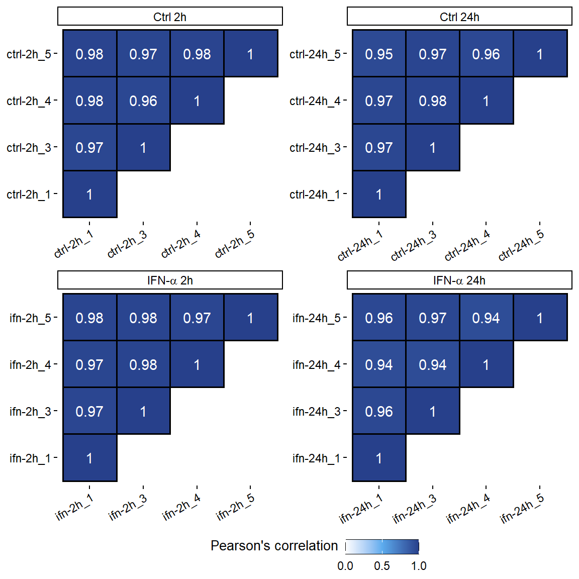
Figure 4: ATAC-seq correlation using the number of reads in a 10kb binned genome normalized with DESeq2.
Differential analysis
The pipeline for differential analysis of ATAC-seq data consists on calling peaks with MACS2 and then performing differential analysis with DESeq2 Bioconductor package.
Once we have the peaks called for the different conditions, we can merge them to create our final region set that we will use for differential analysis. The peak calling is performed in 4 different bam files:
ctrl-2h.merged.bam.ctrl-24h.merged.bam.ifn-2h.merged.bam.ifn-24h.merged.bam.
Then, we will merge the peaks called for each different experiment into a single file, having two final files: 2h.merged and 24h.merged. Since replicate 2 seems to be of bad quality, we are removing it from this analysis.
Next, using Rsubread and DESeq2, we can easily generate the list of open regions in the samples, including the normalized counts, adjusted p-values and log2 Fold Changes. The steps that we have to follow are:
- Load
narrowPeakdata and convert toSAF(needed forRsubread::featureCounts). - Obtain counts for each sample in each region using
Rsubread::featureCounts. - Create
DESeqDataSetobject including annotation data. - Perform differential analysis, obtain results and counts and save into a
data.frame.
## 2 HOURS
## Create SAF with open chromatin regions
saf.2h <- data.frame(peaks.2h)[,1:3]
saf.2h$id <- paste0("region_", 1:nrow(saf.2h))
colnames(saf.2h) <- c("Chr", "Start", "End", "GeneID")
saf.2h$Strand <- "+"
saf.2h <- saf.2h[saf.2h$Chr!="chrX" & saf.2h$Chr!="chrY",]

## Obtain counts in regions
bam.2h <- list.files("../../data/ATAC-seq/BAMs", full.names=TRUE,
                  pattern="*2h_[0-9]\\.bam$")[-c(2,7)]
counts.2h <- Rsubread::featureCounts(bam.2h,
                                  annot.ext=saf.2h,
                                  nthreads=6)
save(counts.2h, file="data/counts.2h.rsubread.rda")

## 24 HOURS
## Create SAF with open chromatin regions
saf.24h <- data.frame(peaks.24h)[,1:3]
saf.24h$id <- paste0("region_", 1:nrow(saf.24h))
colnames(saf.24h) <- c("Chr", "Start", "End", "GeneID")
saf.24h$Strand <- "+"
saf.24h <- saf.24h[saf.24h$Chr!="chrX" & saf.24h$Chr!="chrY",]

## Obtain counts in regions
bam.24h <- list.files("../../data/ATAC-seq/BAMs", full.names=TRUE,
                  pattern="*24h_[0-9]\\.bam$")[-c(2,7)]
counts.24h <- Rsubread::featureCounts(bam.24h,
                                  annot.ext=saf.24h,
                                  nthreads=6)
save(counts.24h, file="../data/IFNa/ATAC/diffAnalysis/counts.24h.rsubread.rda")
## Create DDS object and perform analysis
cts.2h <- counts.2h$counts
colnames(cts.2h) <- names.2h
save(cts.2h, file="../data/IFNa/ATAC/diffAnalysis/counts.2h.matrix.rda")
coldata.2h <- data.frame("treatment"=gsub("_[0-9]", "", names.2h))
library(DESeq2)
dds.2h <- DESeqDataSetFromMatrix(countData = cts.2h,
colData = coldata.2h,
design= ~ treatment)
library("BiocParallel")
register(MulticoreParam(6))
dds.2h <- DESeq(dds.2h, parallel=TRUE)
save(dds.2h, file="../data/IFNa/ATAC/diffAnalysis/dds.2h.rda")
res.2h <- results(dds.2h)
## 24 HOURS
cts.24h <- counts.24h$counts
colnames(cts.24h) <- names.24h
save(cts.24h, file="../data/IFNa/ATAC/diffAnalysis/counts.24h.matrix.rda")
coldata.24h <- data.frame("treatment"=gsub("_[0-9]", "", names.24h))
library(DESeq2)
dds.24h <- DESeqDataSetFromMatrix(countData = cts.24h,
colData = coldata.24h,
design= ~ treatment)
library("BiocParallel")
register(MulticoreParam(6))
dds.24h <- DESeq(dds.24h, parallel=TRUE)
save(dds.24h, file="../data/IFNa/ATAC/diffAnalysis/dds.24h.rda")
res.24h <- results(dds.24h)
res.2h.df <- data.frame(res.2h)
res.24h.df <- data.frame(res.24h)
counts.2h <- counts(dds.2h, normalized=TRUE)
counts.2h <- data.frame(counts.2h)
counts.24h <- counts(dds.24h, normalized=TRUE)
counts.24h <- data.frame(counts.24h)
res.2h.df <- merge(res.2h.df, counts.2h, by="row.names")
res.24h.df <- merge(res.24h.df, counts.24h, by="row.names")
res.2h.df <- res.2h.df[res.2h.df$baseMean!=0,]
res.24h.df <- res.24h.df[res.24h.df$baseMean!=0,]
## Classify regions
res.2h.df$type <- "stable"
res.2h.df$type[res.2h.df$padj<=0.05 & res.2h.df$log2FoldChange>=1] <- "gained"
res.2h.df$type[res.2h.df$padj<=0.05 & res.2h.df$log2FoldChange<=-1] <- "lost"
res.24h.df$type <- "stable"
res.24h.df$type[res.24h.df$padj<=0.05 & res.24h.df$log2FoldChange>=1] <- "gained"
res.24h.df$type[res.24h.df$padj<=0.05 & res.24h.df$log2FoldChange<=-1] <- "lost"
## Add coordinates
colnames(res.2h.df)[1] <- "GeneID"
res.2h.df <- merge(res.2h.df, saf.2h)
res.2h.df <- res.2h.df[!(is.na(res.2h.df$padj)),]
save(res.2h.df, file="../data/IFNa/ATAC/diffAnalysis/res.2h.rda")
colnames(res.24h.df)[1] <- "GeneID"
res.24h.df <- merge(res.24h.df, saf.24h)
res.24h.df <- res.24h.df[!(is.na(res.24h.df$padj)),]
save(res.24h.df, file="../data/IFNa/ATAC/diffAnalysis/res.24h.rda")
res.2h.gr <- regioneR::toGRanges(res.2h.df[,c(17:19,1:7,16)])
save(res.2h.gr, file="../data/IFNa/ATAC/diffAnalysis/res_2h_granges.rda")
res.24h.gr <- regioneR::toGRanges(res.24h.df[,c(17:19,1:7,16)])
save(res.24h.gr, file="../data/IFNa/ATAC/diffAnalysis/res_24h_granges.rda")load("../data/IFNa/ATAC/diffAnalysis/res_2h_granges.rda")
h2 <- res.gr
h2$time <- "2 hours"
load("../data/IFNa/ATAC/diffAnalysis/res_24h_granges.rda")
h24 <- res.gr
h24$time <- "24 hours"
res.gr <- c(h2, h24)
## Get coding genes list
library(biomaRt)
grch37 <- useMart(biomart="ENSEMBL_MART_ENSEMBL",
host="grch37.ensembl.org",
path="/biomart/martservice",
dataset="hsapiens_gene_ensembl")
genes <- getBM(attributes=c("chromosome_name", "start_position", "end_position",
"ensembl_gene_id", "external_gene_name"),
filters="biotype", values="protein_coding",
mart=grch37)
genes <- regioneR::toGRanges(genes)
genes <- genes[seqnames(genes) %in% c(1:22, "X", "Y"),]
seqlevelsStyle(genes) <- "UCSC"
## Annotate ATAC-seq regions to nearest gene
anno <- data.frame(ChIPseeker::annotatePeak(res.gr, TxDb=genes))
anno <- anno[,c(6,14,22,20:21)]
mcols(res.gr) <- dplyr::left_join(as.data.frame(mcols(res.gr)), anno, by=c(GeneID="GeneID", time="time"))
res.gr$annotation <- "Promoter"
res.gr$annotation[abs(res.gr$distanceToTSS)>2e3] <- "Distal"
save(res.gr, file="../data/IFNa/ATAC/diffAnalysis/res_2+24h_anno.rda")load("../data/IFNa/ATAC/diffAnalysis/res_2+24h_anno.rda")
table(res.gr[res.gr$time=="2 hours"]$type, res.gr$annotation[res.gr$time=="2 hours"]) %>%
knitr::kable(format="html",
format.args = list(big.mark = ","),
caption = "Number of regions classified according to significance and distance to TSS in ATAC-seq EndoC samples (2 hours).") %>%
kable_styling(full_width = TRUE) %>%
add_header_above(c("Region type" = 1, "Location respect TSS" = 2))| Distal | Promoter | |
|---|---|---|
| gained | 4,326 | 89 |
| lost | 1 | 0 |
| stable | 248,620 | 13,651 |
table(res.gr[res.gr$time=="24 hours"]$type, res.gr$annotation[res.gr$time=="24 hours"]) %>%
  knitr::kable(format="html",
               format.args = list(big.mark = ","),
               caption = "Number of regions classified according to significance and distance to TSS in ATAC-seq EndoC samples (24 hours).") %>%
  kable_styling(full_width = TRUE) %>%
add_header_above(c("Region type" = 1, "Location respect TSS" = 2))| Distal | Promoter | |
|---|---|---|
| gained | 974 | 26 |
| lost | 9 | 0 |
| stable | 275,709 | 13,558 |
volc_ec <-
  ggplot(data.frame(res.gr),
       aes(log2FoldChange, -log10(padj))) +
  geom_point(aes(color=type), size=0.4) +
  scale_color_manual(values=pals$differential,
                    name="OCR type") +
  geom_vline(xintercept=c(1,-1), linetype=2, color="dark grey") +
  geom_hline(yintercept=-log10(0.05), linetype=2, color="dark grey") +
  xlab(expression(Log[2]*" fold-change")) + ylab(expression(-Log[10]*" FDR adjusted P")) +
  ggtitle(expression("ATAC-seq EndoC-"*beta*H1)) +
  facet_wrap(~time) +
  theme(legend.position="none")

volc_ec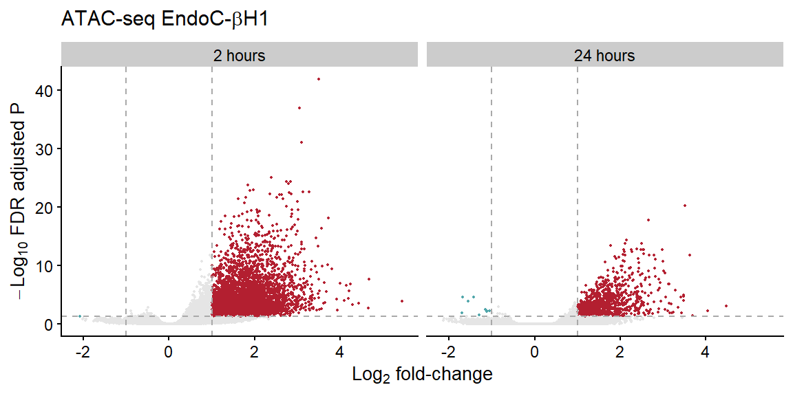
Characterization of OCRs
Distance to TSS
load("../data/IFNa/ATAC/diffAnalysis/res_2+24h_anno.rda")
re.df <- as.data.frame(res.gr)

## Make groups
re.tss <- unique(re.df[!is.na(re.df$type),])

re.tss$anno.group <- NA
re.tss$anno.group[abs(re.tss$distanceToTSS)>200e3] <- ">200kb"
re.tss$anno.group[abs(re.tss$distanceToTSS)<=200e3 &
                    abs(re.tss$distanceToTSS)>20e3] <- "20-200kb"
re.tss$anno.group[abs(re.tss$distanceToTSS)<=20e3 &
                    abs(re.tss$distanceToTSS)>2e3] <- "2-20kb"
re.tss$anno.group[abs(re.tss$distanceToTSS)<=2e3] <- "0-2kb"

## Calculate percentages
len.g_2h <- sum(grepl("gained", re.tss$type) & grepl("2 hours", re.tss$time))
len.s_2h <- sum(grepl("stable", re.tss$type) & grepl("2 hours", re.tss$time))
len.g_24h <- sum(grepl("gained", re.tss$type) & grepl("24 hours", re.tss$time))
len.s_24h <- sum(grepl("stable", re.tss$type) & grepl("24 hours", re.tss$time))

sum.tss <- re.tss %>%
  group_by(type, anno.group, time) %>%
  summarise(num=length(unique(GeneID)))

sum.tss$perc <- NA
sum.tss$perc[grepl("gained", sum.tss$type) & grepl("2 hours", sum.tss$time)] <- sum.tss$num[grepl("gained", sum.tss$type) & grepl("2 hours", sum.tss$time)]/len.g_2h*100
sum.tss$perc[grepl("stable", sum.tss$type) & grepl("2 hours", sum.tss$time)] <- sum.tss$num[grepl("stable", sum.tss$type) & grepl("2 hours", sum.tss$time)]/len.s_2h*100
sum.tss$perc[grepl("gained", sum.tss$type) & grepl("24 hours", sum.tss$time)] <- sum.tss$num[grepl("gained", sum.tss$type) & grepl("24 hours", sum.tss$time)]/len.g_24h*100
sum.tss$perc[grepl("stable", sum.tss$type) & grepl("24 hours", sum.tss$time)] <- sum.tss$num[grepl("stable", sum.tss$type) & grepl("24 hours", sum.tss$time)]/len.s_24h*100

sum.tss$anno.group <- factor(sum.tss$anno.group,
                             levels=c("0-2kb", "2-20kb", "20-200kb", ">200kb"))

tss.plot <-
  ggplot(sum.tss[sum.tss$type %in% c("gained", "stable"),],
       aes(anno.group, perc)) +
  geom_bar(aes(fill=type), color="black", lwd=0.7, stat="identity", position="dodge") +
  geom_vline(xintercept=1.5, lty=2, color="dark red") +
  scale_fill_manual(values=pals$differential,
                    name="OCR type") +
  theme(legend.position="top") +
  xlab("Distance to TSS") +
  scale_y_continuous(name="Percentage of RE",
                     labels=function(x) paste0(x, "%"),
                     breaks=scales::pretty_breaks()) +
  facet_wrap(~time)

tss.plot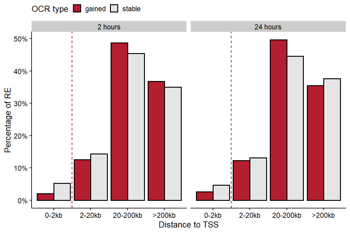
Figure 5: Distribution of OCRs according to their distance to the nearest TSS.
Sequence conservation
library(GenomicRanges)
library(pipelineNGS)

path_bw <- "C:/Users/mirei/Documents/data/phastCons_46_placentalMammals/placental_mammals.bw"

scope <- 1e3
bin <- 25

load("../data/IFNa/ATAC/diffAnalysis/res_2h_granges.rda")
res.2h.gr <- res.gr
g2h <- res.2h.gr[res.2h.gr$type=="gained",]
g2h.cons <- calculateMeanCons(g2h,
                              scope=scope, bin=bin,
                              phastConsBW = path_bw)
g2h.cons$type <- "gained"
g2h.cons$time <- "2h"

g2h.rnd <- regioneR::randomizeRegions(g2h,
                                       allow.overlaps = FALSE)
g2h.rnd.cons <- calculateMeanCons(g2h.rnd,
                              scope=scope, bin=bin,
                              phastConsBW = path_bw)
g2h.rnd.cons$type <- "random"
g2h.rnd.cons$time <- "2h"

load("../data/IFNa/ATAC/diffAnalysis/res_24h_granges.rda")
res.24h.gr <- res.gr
g24h <- res.24h.gr[res.24h.gr$type=="gained",]
g24h.cons <- calculateMeanCons(g24h,
                              scope=scope, bin=bin,
                              phastConsBW = path_bw)
g24h.cons$type <- "gained"
g24h.cons$time <- "24h"

g24h.rnd <- regioneR::randomizeRegions(g24h,
                                       allow.overlaps = FALSE)
g24h.rnd.cons <- calculateMeanCons(g24h.rnd,
                              scope=scope, bin=bin,
                              phastConsBW = path_bw)
g24h.rnd.cons$type <- "random"
g24h.rnd.cons$time <- "24h"

g.cons <- rbind(g2h.cons, g2h.rnd.cons,
                g24h.cons, g24h.rnd.cons)

g.cons$time <- factor(g.cons$time, levels=c("2h", "24h"))
save(g.cons, file=file.path(out_dir, "IFN_conservation.rda"))
load(file.path(out_dir, "IFN_conservation.rda"))
ggplot(g.cons) +
geom_line(aes(position, meanCons, color=type, group=type),
lwd=0.7) +
facet_wrap(~time) +
scale_color_discrete(name="Region type",
labels=function(x) Hmisc::capitalize(x)) +
xlab("Position from peak center (bp)") +
ylab("Mean PhastCons46way score") +
theme(legend.position="top")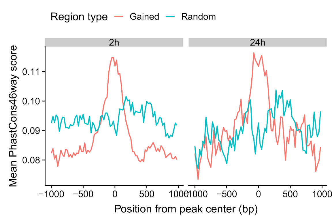
Figure 6: Mean phastCons sequence conservation scores of gained OCRs.
de Novo TF Motifs
Note: This analysis has been re-run and thus, results might slightly differ from the ones presented in the original publication, as the de Novo motif finding includes some randomicity in its calculations. However, the main results, that is, the finding of both inflammatory and islet-specific TFs in gained OCRs is still maintained.
library(maRge)

out_homer <- file.path(out_dir, "motifs_2h_gained/")

deNovoMotifHOMER(bed=paste0("../data/IFNa/bedfiles/OCRs_gained_2h.bed"),
                 path_output=out_homer,
                 other_param="-mask",
                 path_homer="~/tools/homer/")
htmltools::includeHTML(file.path(out_dir, "motifs_2h_gained/homerResults.html"))Homer de novo Motif Results (motifs_2h_gained/)
Known Motif Enrichment ResultsGene Ontology Enrichment Results
If Homer is having trouble matching a motif to a known motif, try copy/pasting the matrix file into STAMP
More information on motif finding results: HOMER | Description of Results | Tips
Total target sequences = 4415
Total background sequences = 45308
* - possible false positive
| Rank | Motif | P-value | log P-pvalue | % of Targets | % of Background | STD(Bg STD) | Best Match/Details | Motif File |
| 1 | 1e-4327 | -9.965e+03 | 70.53% | 1.74% | 139.8bp (137.7bp) | IRF1(IRF)/PBMC-IRF1-ChIP-Seq(GSE43036)/Homer(0.996) More Information | Similar Motifs Found | motif file (matrix) | |
| 2 | 1e-260 | -5.996e+02 | 22.88% | 6.67% | 204.0bp (138.3bp) | Arnt:Ahr(bHLH)/MCF7-Arnt-ChIP-Seq(Lo_et_al.)/Homer(0.664) More Information | Similar Motifs Found | motif file (matrix) | |
| 3 | 1e-47 | -1.087e+02 | 10.69% | 5.19% | 195.2bp (137.8bp) | PB0035.1_Irf5_1/Jaspar(0.838) More Information | Similar Motifs Found | motif file (matrix) | |
| 4 | 1e-40 | -9.421e+01 | 25.89% | 17.73% | 207.4bp (139.4bp) | EWS:FLI1-fusion(ETS)/SK_N_MC-EWS:FLI1-ChIP-Seq(SRA014231)/Homer(0.763) More Information | Similar Motifs Found | motif file (matrix) | |
| 5 | 1e-36 | -8.315e+01 | 3.67% | 1.13% | 157.1bp (142.6bp) | IRF7/MA0772.1/Jaspar(0.635) More Information | Similar Motifs Found | motif file (matrix) | |
| 6 | 1e-29 | -6.879e+01 | 1.34% | 0.19% | 142.4bp (119.4bp) | PH0037.1_Hdx/Jaspar(0.643) More Information | Similar Motifs Found | motif file (matrix) | |
| 7 | 1e-27 | -6.255e+01 | 1.06% | 0.13% | 117.6bp (110.6bp) | CEBPA/MA0102.3/Jaspar(0.806) More Information | Similar Motifs Found | motif file (matrix) | |
| 8 | 1e-26 | -6.038e+01 | 1.25% | 0.19% | 99.5bp (127.3bp) | Rfx5(HTH)/GM12878-Rfx5-ChIP-Seq(GSE31477)/Homer(0.816) More Information | Similar Motifs Found | motif file (matrix) | |
| 9 | 1e-25 | -5.789e+01 | 0.32% | 0.00% | 146.2bp (0.0bp) | NFY(CCAAT)/Promoter/Homer(0.686) More Information | Similar Motifs Found | motif file (matrix) | |
| 10 | 1e-25 | -5.758e+01 | 20.57% | 14.73% | 183.5bp (141.4bp) | AP-1(bZIP)/ThioMac-PU.1-ChIP-Seq(GSE21512)/Homer(0.960) More Information | Similar Motifs Found | motif file (matrix) | |
| 11 | 1e-23 | -5.374e+01 | 9.01% | 5.30% | 170.2bp (131.3bp) | RUNX1(Runt)/Jurkat-RUNX1-ChIP-Seq(GSE29180)/Homer(0.777) More Information | Similar Motifs Found | motif file (matrix) | |
| 12 | 1e-22 | -5.281e+01 | 28.29% | 21.89% | 195.6bp (139.7bp) | Foxo1(Forkhead)/RAW-Foxo1-ChIP-Seq(Fan_et_al.)/Homer(0.974) More Information | Similar Motifs Found | motif file (matrix) | |
| 13 | 1e-21 | -4.874e+01 | 1.56% | 0.38% | 143.2bp (126.1bp) | PGR(NR)/EndoStromal-PGR-ChIP-Seq(GSE69539)/Homer(0.624) More Information | Similar Motifs Found | motif file (matrix) | |
| 14 | 1e-20 | -4.803e+01 | 0.27% | 0.00% | 154.9bp (47.8bp) | PB0187.1_Tcf7_2/Jaspar(0.687) More Information | Similar Motifs Found | motif file (matrix) | |
| 15 | 1e-19 | -4.502e+01 | 13.48% | 9.24% | 196.4bp (138.5bp) | Gata1(Zf)/K562-GATA1-ChIP-Seq(GSE18829)/Homer(0.948) More Information | Similar Motifs Found | motif file (matrix) | |
| 16 | 1e-19 | -4.480e+01 | 26.50% | 20.75% | 207.4bp (137.3bp) | PDX1/Human-Islets(0.844) More Information | Similar Motifs Found | motif file (matrix) | |
| 17 | 1e-18 | -4.320e+01 | 0.39% | 0.01% | 62.8bp (88.0bp) | PH0139.1_Pitx3/Jaspar(0.621) More Information | Similar Motifs Found | motif file (matrix) | |
| 18 | 1e-17 | -4.014e+01 | 20.82% | 15.89% | 203.2bp (142.5bp) | PU.1(ETS)/ThioMac-PU.1-ChIP-Seq(GSE21512)/Homer(0.762) More Information | Similar Motifs Found | motif file (matrix) | |
| 19 | 1e-17 | -4.008e+01 | 21.40% | 16.42% | 189.1bp (143.6bp) | SCL(bHLH)/HPC7-Scl-ChIP-Seq(GSE13511)/Homer(0.798) More Information | Similar Motifs Found | motif file (matrix) | |
| 20 | 1e-17 | -4.007e+01 | 0.97% | 0.18% | 117.7bp (121.9bp) | ESRRB/MA0141.3/Jaspar(0.651) More Information | Similar Motifs Found | motif file (matrix) | |
| 21 | 1e-17 | -3.964e+01 | 1.34% | 0.34% | 150.9bp (144.2bp) | MZF1/MA0056.1/Jaspar(0.644) More Information | Similar Motifs Found | motif file (matrix) | |
| 22 | 1e-17 | -3.946e+01 | 1.22% | 0.29% | 133.9bp (127.5bp) | POL004.1_CCAAT-box/Jaspar(0.694) More Information | Similar Motifs Found | motif file (matrix) | |
| 23 | 1e-17 | -3.928e+01 | 0.61% | 0.06% | 135.8bp (144.8bp) | Arnt:Ahr(bHLH)/MCF7-Arnt-ChIP-Seq(Lo_et_al.)/Homer(0.632) More Information | Similar Motifs Found | motif file (matrix) | |
| 24 | 1e-15 | -3.572e+01 | 31.12% | 25.68% | 222.7bp (139.2bp) | Atoh1(bHLH)/Cerebellum-Atoh1-ChIP-Seq(GSE22111)/Homer(0.693) More Information | Similar Motifs Found | motif file (matrix) | |
| 25 | 1e-15 | -3.502e+01 | 0.27% | 0.01% | 74.3bp (79.0bp) | RUNX-AML(Runt)/CD4+-PolII-ChIP-Seq(Barski_et_al.)/Homer(0.687) More Information | Similar Motifs Found | motif file (matrix) | |
| 26 | 1e-14 | -3.450e+01 | 13.59% | 9.84% | 194.3bp (140.5bp) | ZBTB12(Zf)/HEK293-ZBTB12.GFP-ChIP-Seq(GSE58341)/Homer(0.625) More Information | Similar Motifs Found | motif file (matrix) | |
| 27 | 1e-14 | -3.441e+01 | 18.17% | 13.87% | 203.3bp (141.5bp) | POL010.1_DCE_S_III/Jaspar(0.722) More Information | Similar Motifs Found | motif file (matrix) | |
| 28 | 1e-13 | -3.164e+01 | 0.23% | 0.01% | 54.2bp (149.5bp) | PB0207.1_Zic3_2/Jaspar(0.650) More Information | Similar Motifs Found | motif file (matrix) | |
| 29 | 1e-13 | -3.023e+01 | 41.13% | 35.74% | 212.0bp (139.4bp) | ZNF354C/MA0130.1/Jaspar(0.678) More Information | Similar Motifs Found | motif file (matrix) | |
| 30 | 1e-12 | -2.770e+01 | 0.20% | 0.01% | 100.4bp (47.5bp) | E2A(bHLH)/proBcell-E2A-ChIP-Seq(GSE21978)/Homer(0.711) More Information | Similar Motifs Found | motif file (matrix) | |
| 31 | 1e-12 | -2.770e+01 | 0.20% | 0.01% | 139.7bp (88.8bp) | PB0099.1_Zfp691_1/Jaspar(0.645) More Information | Similar Motifs Found | motif file (matrix) | |
| 32 | 1e-12 | -2.770e+01 | 0.20% | 0.01% | 130.9bp (121.8bp) | Barhl1/MA0877.1/Jaspar(0.577) More Information | Similar Motifs Found | motif file (matrix) | |
| 33 * | 1e-11 | -2.604e+01 | 6.46% | 4.23% | 196.6bp (135.6bp) | YY1/MA0095.2/Jaspar(0.666) More Information | Similar Motifs Found | motif file (matrix) | |
| 34 * | 1e-11 | -2.551e+01 | 1.36% | 0.49% | 153.7bp (121.8bp) | Brn2(POU,Homeobox)/NPC-Brn2-ChIP-Seq(GSE35496)/Homer(0.622) More Information | Similar Motifs Found | motif file (matrix) | |
| 35 * | 1e-10 | -2.386e+01 | 0.18% | 0.01% | 78.7bp (111.6bp) | SP1/MA0079.3/Jaspar(0.735) More Information | Similar Motifs Found | motif file (matrix) | |
| 36 * | 1e-8 | -2.049e+01 | 0.36% | 0.05% | 178.1bp (132.4bp) | ZNF354C/MA0130.1/Jaspar(0.719) More Information | Similar Motifs Found | motif file (matrix) | |
| 37 * | 1e-8 | -2.040e+01 | 0.34% | 0.04% | 126.6bp (147.4bp) | Twist2/MA0633.1/Jaspar(0.770) More Information | Similar Motifs Found | motif file (matrix) | |
| 38 * | 1e-7 | -1.806e+01 | 30.69% | 26.93% | 215.9bp (138.5bp) | NKX2-8/MA0673.1/Jaspar(0.680) More Information | Similar Motifs Found | motif file (matrix) |